In this section, we present in detail the treatment
of vector meson contributions to some anomalous processes of interest and
show that in the anomalous sector, within the resonance saturation
hypothesis, one can get unambiguous predictions for the renormalized
parameters of the low energy effective Lagrangian. We shall start
with the general discussion of the amplitude for
 , indicate its extension to the
virtual photon case
, indicate its extension to the
virtual photon case  in more
detail than in the first section, discuss
modifications due to counterterms and their
saturation with vector mesons , and then illustrate the introduction in the
chiral lagrangian of
vector meson fields as from the Hidden Symmetry approach. The resulting lagrangian
contains three parameters which we show to be related to the usual
chiral perturbative counterterms.
Examining processes like
in more
detail than in the first section, discuss
modifications due to counterterms and their
saturation with vector mesons , and then illustrate the introduction in the
chiral lagrangian of
vector meson fields as from the Hidden Symmetry approach. The resulting lagrangian
contains three parameters which we show to be related to the usual
chiral perturbative counterterms.
Examining processes like  with the photon on or off the masss shell, we
are able to indicate a range of variability for these parameters and
will then proceed to calculate the cross-section for
the three processes
with the photon on or off the masss shell, we
are able to indicate a range of variability for these parameters and
will then proceed to calculate the cross-section for
the three processes 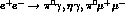 .
.
We focus our attention to the next-to-leading effective chiral Lagrangian describing the interaction of photons with pseudoscalars. Explicitly, the relevant part of the lowest-order anomalous Lagrangian is
where the dots refer to non-photonic terms, irrelevant for our present purposes,
and the whole nonet of pseudoscalar mesons (with the phenomenologically
preferred  -
- mixing angle
  ) now appears in
  through the matrix
  defined in the first section.
>From the first term in (25) one immediately deduces the amplitude for
the  decay to order
  , i.e.
which successfully predicts  eV for f=132 MeV. Similarly, one
obtains a good description of
eV for f=132 MeV. Similarly, one
obtains a good description of  ,
,  decays as
shown in ref.[12] for the above value of
decays as
shown in ref.[12] for the above value of  .
.
While this amplitude is finite, this result
no longer holds
when dealing with off-mass-shell photon(s), as in the  ,
,  production or in the
  ,
,
 decay amplitudes.
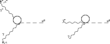
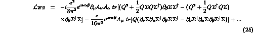
Figure 1: Loop diagrams contributing to  processes at order
In these cases, diagrams like the ones in Fig.(1) give a contribution whose divergence is cancelled by a corresponding counterterm in the relevant order six lagrangian, i.e. [12]
where  and
and  are constants to be determined. Calling
 and
and  the finite part of loop and counterterm corrections, the
resulting amplitude is now written as [12]
the finite part of loop and counterterm corrections, the
resulting amplitude is now written as [12]
where,  ,
,  ,
,  and, neglecting
the small effects originated by the
and, neglecting
the small effects originated by the  singlet part in the physical
 wave function,
with  defined as
The
finite parts of the loop and counterterm
corrections depend on the renormalization mass scale  . This will be
fixed around the
. This will be
fixed around the  - and
- and  -meson masses,
  ,
which are the relevant ones in our case.
Then eq.(29) for
,
which are the relevant ones in our case.
Then eq.(29) for  reduces to
As for the counterterm contribution, from eq.(27) one immediately has
The numerical value of (32) can be fixed from
experiments on  decays [13] or (better) from
a recent
experiment on
decays [13] or (better) from
a recent
experiment on  production through one (essentially)
real photon and a virtual one [7]. The measured
production through one (essentially)
real photon and a virtual one [7]. The measured  -dependence
of the
amplitude can be linearly parametrized in terms of a
slope parameter
-dependence
of the
amplitude can be linearly parametrized in terms of a
slope parameter
 , i.e.
Using also (31) and (32) one has [7]
By comparig this experimental result with the contribution from the loops (28), the counterterms contribution turns out to be dominant and given by
Similarly, a single measurement using  leads to
 , thus confirming eqs.(34)
and (35) (see Ametller's contribution to this Handbook).
, thus confirming eqs.(34)
and (35) (see Ametller's contribution to this Handbook).
The experimental results just described,
and their parameterization in terms of  ,
can now be used to test the saturation hypothesis of the counterterms by
resonance exchange. Let us introduce in this context
the whole nonet of vector mesons, V,
as gauge bosons of the HS-model of Bando and collaborators
[14,2].
At order
,
can now be used to test the saturation hypothesis of the counterterms by
resonance exchange. Let us introduce in this context
the whole nonet of vector mesons, V,
as gauge bosons of the HS-model of Bando and collaborators
[14,2].
At order  , the relevant lagrangian
(which can be found in ref. [12]) can be written as
a linear combination of three independent
terms with coefficients
, the relevant lagrangian
(which can be found in ref. [12]) can be written as
a linear combination of three independent
terms with coefficients  . As it turns out,
only terms proportional
to the constants
. As it turns out,
only terms proportional
to the constants  and
and  are relevant to
the processes we are interested here, while all
three enter
into the study of a process like
are relevant to
the processes we are interested here, while all
three enter
into the study of a process like  , discussed
in refs.[15,16].
Including also the
first term from
, discussed
in refs.[15,16].
Including also the
first term from  (25),
the pieces of the whole Lagrangian relevant to
(25),
the pieces of the whole Lagrangian relevant to
 ,
,  and VVP vertices are written as
Vector meson mass terms and standard  couplings
appear in the lagrangian
couplings
appear in the lagrangian
with the constants g and f satisfying the relations
 and the lagrangian
  generalizing
eq.(18) with
generalizing
eq.(18) with
The above contributions to the lagrangian are such that
only the first term in  , i.e. the first term in
 , contributes to
the
, contributes to
the  amplitude for real photons. Indeed
once the
amplitude for real photons. Indeed
once the  transition
(37) is used in eq.(36) there is a
cancellation of all
transition
(37) is used in eq.(36) there is a
cancellation of all  dependent terms and one
recovers the results of
eq.(26).
The
dependent terms and one
recovers the results of
eq.(26).
The  dependence appears when dealing with
vertices such as
dependence appears when dealing with
vertices such as  ,
,  or
or
 ,
,  , where the
virtual photon introduces also a
, where the
virtual photon introduces also a  -dependence through the vector
meson form-factor
-dependence through the vector
meson form-factor  .
Expanding in powers of
.
Expanding in powers of  and retaining up to the second term,
we can now compare
the vector meson contributions from the above lagrangian (given
in terms of
and retaining up to the second term,
we can now compare
the vector meson contributions from the above lagrangian (given
in terms of  ) with
the
) with
the  coefficients in
  , eq.(27)
. As shown in [12], one easily obtains
, eq.(27)
. As shown in [12], one easily obtains
The actual numerical values for the above constants can be deduced from
the experimental data relative to a  process
like the decay
process
like the decay
 . The measured width
 keV
keV  [13] leads to
in good agreement with (35), thus confirming the resonance saturation
hypothesis for the counterterms,  .
.
Let us now discuss the relationship between the above
lagrangians eqs.( 36-37) and the
vector meson dominance model, in which no direct
coupling between pseudoscalar mesons and photons appears. This result is
easily obtained with the following choice of parameters  and
and 
which eliminates all direct  and
and  vertices in the Lagrangian (36). The relative decay vertices are
then exclusively generated by the
vertices in the Lagrangian (36). The relative decay vertices are
then exclusively generated by the  term and
 conversion(s) from
  as in conventional
VMD, indicating the consistency of the latter with
the model of
Bando et al.[14,2] for the above choice of the parameters
as in conventional
VMD, indicating the consistency of the latter with
the model of
Bando et al.[14,2] for the above choice of the parameters
 and
and  .
However, the agreement between eq.(35) and eqs.(39)and
(40),
which confirms the saturation hypothesis
for the Bando model, does not fix the individual values
of
.
However, the agreement between eq.(35) and eqs.(39)and
(40),
which confirms the saturation hypothesis
for the Bando model, does not fix the individual values
of  and
and  , but only the sum
  . The choice
can then be adopted to include both the VMD conventional model, for which
eq.(41) is satisfied, as well as
deviations from this model through  ,
while still satisfying eq.(40).
,
while still satisfying eq.(40).
The
possibility of deviations from VMD has been discussed in the related
context of  transitions[15]. Other informations can be
extracted from experimental data on the decays
transitions[15]. Other informations can be
extracted from experimental data on the decays
 [17] where the
  -dependence has been
parametrized in terms of the usual e.m.
transition
form-factor
-dependence has been
parametrized in terms of the usual e.m.
transition
form-factor  (see
Ll.Ametller in this Handbook).
The data can be fitted with
(see
Ll.Ametller in this Handbook).
The data can be fitted with  and seem to indicate a deviation from the
usual vector meson dominance, for which one would have chosen
and seem to indicate a deviation from the
usual vector meson dominance, for which one would have chosen
 . Such discrepancy can
easily be explained in terms
of the Lagrangians (36) and (37), which imply a form-factor
given by
. Such discrepancy can
easily be explained in terms
of the Lagrangians (36) and (37), which imply a form-factor
given by
Comparing eq.(43) with
 ,
we see that experimental data imply
,
we see that experimental data imply  and,
up to this order, a good choice
seems to be
and,
up to this order, a good choice
seems to be
 . This is however not a completely
unambiguous choice. If one is willing to extend this
formalism to higher
. This is however not a completely
unambiguous choice. If one is willing to extend this
formalism to higher  , the
data [17] tend to prefer values of
, the
data [17] tend to prefer values of  somewhat larger than
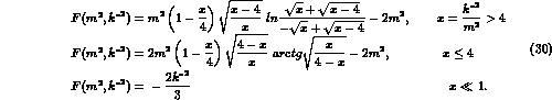
 , as one can see from Fig.(2), where we plot the fits for the
 -dependence of the form factor in
  for the experimental case and two different choices of the parameters.
We see that we can adopt
as a compromise which represents an interesting alternative to the VMD values (41).
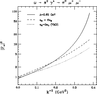
Figure 2: Fits to the  -dependence of the form-factor in
  . The data (not shown) are compatible with
the solid and dashed lines but not with VMD .
. The data (not shown) are compatible with
the solid and dashed lines but not with VMD .
Apart from giving a reasonable description of the
 data, the
values (44) are also in the preferred region in
order to account for the data on the
data, the
values (44) are also in the preferred region in
order to account for the data on the  . This has
been discussed in detail in refs.[15,16], and the result can be
summarized in Fig.(3),
where values of the parameters
. This has
been discussed in detail in refs.[15,16], and the result can be
summarized in Fig.(3),
where values of the parameters  and
and  consistent with
experimental data are plotted.
consistent with
experimental data are plotted.
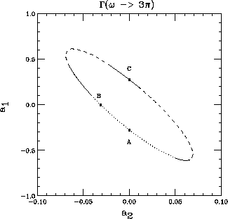
Figure 3: The ellipse defines the values of parameters  and
and  which give the correct width for the
  within
one (dots), two (full) or more (dashes) standard
deviations from the data for
within
one (dots), two (full) or more (dashes) standard
deviations from the data for
 cross-section near the
  peak.
The choices A and C are discussed in [15].
peak.
The choices A and C are discussed in [15].
The branching ratios for
 and
and  fix
a region in the
fix
a region in the  parameter space, represented by
the ellipse. The point B on the ellipse corresponds
to the value in eq.(44) extracted from the process
parameter space, represented by
the ellipse. The point B on the ellipse corresponds
to the value in eq.(44) extracted from the process
 .
Notice that these values of the parameters
.
Notice that these values of the parameters  , which imply a deviation
from pure VMD, find a partial confirmation in recent analyses of
the
, which imply a deviation
from pure VMD, find a partial confirmation in recent analyses of
the  form-factor in the lattice [18].
To summarize, we have discussed the relationship between conventional
VMD, counterterm contributions in chiral perturbation theory
and a possible model for introduction of vector mesons in the chiral
lagrangian to saturate the counterterms. To clarify some of the issues
involved, such as the
presence of a possible clear deviation from
VMD, we now proceed to calculate the
production cross-sections for the reactions
 and
and  which can be measured at DA
 NE and might improve the whole situation and
contribute to fix the value of the ChPT counterterms or the
NE and might improve the whole situation and
contribute to fix the value of the ChPT counterterms or the  parameters.