So far, we have presented the exact solutions
of the renormalization group equations for the Wilson coefficients. In
practice, it is only possible to calculate the relevant functions in perturbation
theory. For illustrative purposes, we consider
the calculation of the  effective Hamiltonian at the leading order in
QCD. The bare Hamiltonian is given in eq. (29).
In the presence of QCD interactions, other operators appear
in the Wilson expansion.
A complete basis is given by the following operators
effective Hamiltonian at the leading order in
QCD. The bare Hamiltonian is given in eq. (29).
In the presence of QCD interactions, other operators appear
in the Wilson expansion.
A complete basis is given by the following operators
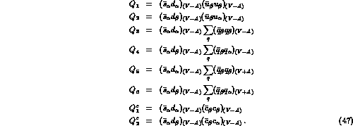
The q index runs over the ``active'' flavours.
The above operators are generated by gluon exchanges
in the Feynman diagrams of fig.
2.
In particular,  is generated by current--current
diagrams and
is generated by current--current
diagrams and  --
-- are generated by penguin diagrams. The
choice of the operator basis in not unique, and different possibilities have
been considered in the literature [27]. If the electromagnetic
correction, are also taken into account, the operator basis enlarges
to include the following operators
are generated by penguin diagrams. The
choice of the operator basis in not unique, and different possibilities have
been considered in the literature [27]. If the electromagnetic
correction, are also taken into account, the operator basis enlarges
to include the following operators

Below the bottom threshold, the following relation holds
so that there are nine independent operators. The basis is further reduced below the charm threshold by using the relations

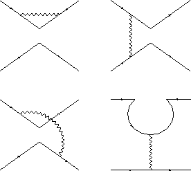
Figure: One-loop corrections to the  effective Hamiltonian.
All the operators considered above are dimension-six operators. In principle, two dimension-five operators
should also be included in the operator basis.
The matrix elements of  and
and
 , however, enter only at
  in chiral perturbation theory. Since the phenomenological analysis
presented in the following is only valid up
to terms of
in chiral perturbation theory. Since the phenomenological analysis
presented in the following is only valid up
to terms of  , we do not need to include the contribution
of the dimension-five operators in the calculation of
, we do not need to include the contribution
of the dimension-five operators in the calculation of  .
The effect of these operators on
.
The effect of these operators on  has recently been
analysed in ref. [29].
Other operators of lower dimensionality
(e.g. two-fermion operators) are also potentially present.
However, it can be shown
that their effect can be reabsorbed in a suitable redefinition
of the fermion fields and by diagonalizing the quark mass matrix
at first order in
has recently been
analysed in ref. [29].
Other operators of lower dimensionality
(e.g. two-fermion operators) are also potentially present.
However, it can be shown
that their effect can be reabsorbed in a suitable redefinition
of the fermion fields and by diagonalizing the quark mass matrix
at first order in  [23]--[26].
In summary, the  effective Hamiltonian, renormalized at a scale
 , can be written as
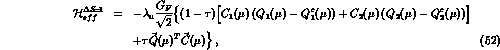
where, in order to find the Wilson coefficients to a given order
in  , we have to calculate eqs.
(41), (45) in perturbation theory.
, we have to calculate eqs.
(41), (45) in perturbation theory.
The explicit expressions of  and
and  ,
in the LLA
,
in the LLA

can be found for example in ref. [5].
In eq. (41), using  and
and  ,
one obtains
,
one obtains

At this order, the matching conditions are trivial:
 , eq. (43), is the identity matrix;
 , eq. (42), has all vanishing components with
the only exception of
, eq. (42), has all vanishing components with
the only exception of  .
Thus the Wilson coefficients at the leading order for
.
Thus the Wilson coefficients at the leading order for
 are given by

with  and all the other Wilson coefficients at the
scale
and all the other Wilson coefficients at the
scale  vanish.
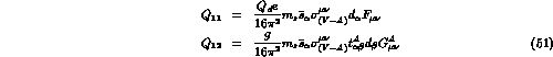
In the next-to-leading logarithmic approximation
(NLLA), one proceeds along the general scheme
described above. In this case, all quantities entering in the
matching procedure have to be computed at order  (
( for the
electromagnetic case). The
for the
electromagnetic case). The  -function and the anomalous dimension
matrix have to be computed at second order in the coupling constants.
Thus, for example,
the anomalous dimension matrix in the NLLA has the form
-function and the anomalous dimension
matrix have to be computed at second order in the coupling constants.
Thus, for example,
the anomalous dimension matrix in the NLLA has the form

where  corrections have been neglected.
We will not give here any details of the NLLA calculations. They
can be found in refs. [1]--[5].
At the next-to-leading order,
it is necessary to solve numerically eq.
(37).
Table 1 contains the coefficients,
calculated at the leading (LO) and at the next-to-leading (NLO) order,
using the 't Hooft--Veltman (HV) and the naïve dimensional (NDR)
regularization
schemes, for different values of the renormalization scale
corrections have been neglected.
We will not give here any details of the NLLA calculations. They
can be found in refs. [1]--[5].
At the next-to-leading order,
it is necessary to solve numerically eq.
(37).
Table 1 contains the coefficients,
calculated at the leading (LO) and at the next-to-leading (NLO) order,
using the 't Hooft--Veltman (HV) and the naïve dimensional (NDR)
regularization
schemes, for different values of the renormalization scale  .
The errors in the table take into account the variation of the
values of the coefficients due to
.
The errors in the table take into account the variation of the
values of the coefficients due to  MeV
and
MeV
and  GeV.
Notice that the next-to-leading Wilson coefficients and operators both depend
on the regularization scheme, while the effective Hamiltonian is
scheme-independent
up to terms
GeV.
Notice that the next-to-leading Wilson coefficients and operators both depend
on the regularization scheme, while the effective Hamiltonian is
scheme-independent
up to terms  . Actually the dependence of the effective
Hamiltonian on the regularization scheme, due to the unknown
next-to-next-to-leading terms, can be estimated and contributes to the
uncertainties in the prediction of
. Actually the dependence of the effective
Hamiltonian on the regularization scheme, due to the unknown
next-to-next-to-leading terms, can be estimated and contributes to the
uncertainties in the prediction of  , see ref. [9].
The coefficients in table 1 have been computed independently by
the Munich group [4,14].
The definition of the renormalized operators in the HV scheme used here
differ from those defined in ref. [14].
This is due to the different way of taking into account the two-loop
anomalous dimension of the weak current, which does not vanish in the HV
calculation. One can relate the HV coefficients of table 1
( ) and those of ref. [14] (
 ). The relation is

where

Once these differences in the definition of the renormalized operators and the reduction of the operator basis, eq. (49), are properly taken into account, the numerical results presented here agree with those of ref. [14].
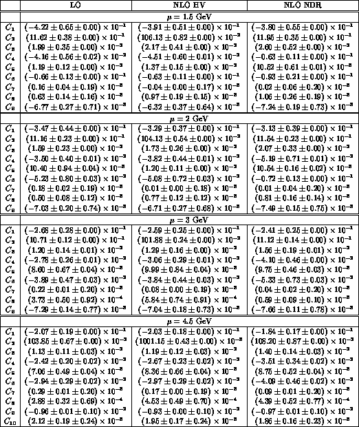
Table: Wilson coefficients of the  effective Hamiltonian
at
effective Hamiltonian
at  GeV. For
  , the relation (49) has been
used to reduce the operator basis.
We take
, the relation (49) has been
used to reduce the operator basis.
We take  MeV and
  GeV.
The values of the coefficients shown here correspond to the central values of
these parameters. The first error is due to the uncertainty on
GeV.
The values of the coefficients shown here correspond to the central values of
these parameters. The first error is due to the uncertainty on  ,
the second is due to
,
the second is due to  .
.
