 amplitudes were performed by Fearing, Fischbach and Smith
[50] using current algebra techniques.
Prior to CHPT, the most detailed calculations of  amplitudes were performed by Fearing, Fischbach and Smith
[50] using current algebra techniques.
In the framework of CHPT, the amplitudes are given by (4.17) and (4.18) to leading order in the chiral expansion.

There are in general three types of contributions [44]:
anomaly, local contributions due to  and loop amplitudes.

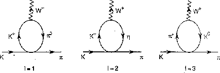
Figure 4.2: Loop diagrams (without tadpoles) for  at
at  . For
. For
 , the photon must be appended on all charged lines and
on all vertices.
The anomaly contributes to the axial amplitudes
The loop diagrams for  are shown in
Fig. 4.2. We first write the
  matrix element
in terms of three functions
  which will also appear
in the invariant amplitudes
  . Including the contributions
from the low-energy constants
  in
in  , the
, the
 matrix element
  is given by
 is a scale independent coupling constant and we have traded
the tadpole contribution together with
  for
for  in
in
 . The sum over I corresponds to the three loop diagrams
of Fig. 4.2 with coefficients
  displayed in
table 4.3.

Table 4.3: Coefficients for the  loop amplitudes
corresponding to the diagrams I=1,2,3 in Fig. 4.2.
All coefficients
  must be divided by
 .
.
We use the Gell-Mann--Okubo mass formula
throughout to express  in terms of
  .
The functions
  and
and  can be found in App. B.
The standard  form factors
  as given in the previous subsection [24] are

It remains to calculate the infrared finite tensor amplitude
 . The invariant amplitudes
  can be
expressed in terms of the previously defined functions
  and of
additional amplitudes
  . Diagrammatically, the latter
amplitudes arise from those diagrams in Fig. 4.2 where the
photon is not appended on the incoming
  (non-Bremsstrahlung
diagrams). The final expressions are
The amplitudes  in Eq.(4.22) are given by
The function  is given in App. B.
All the invariant amplitudes
  are
real in the physical region. Of course, the same is true for the
 matrix element
  .
.
The  amplitude has a very similar structure. Both the
 matrix element
  and the infrared finite
vector amplitude
  can be obtained from the
corresponding quantities
  and
and
 by the following steps:
 and
and  ;
;
 by
by  in
in  ;
;
 for
for
 listed in table 4.4;
 and
and  by a
factor
  .
.

Table 4.4: Coefficients for the  loop amplitudes
corresponding to the diagrams I=1,2,3 in Fig. 4.2. All
coefficients
  must be divided by
  .
.

In calculating the rates with the complete amplitudes of the previous subsection, we use the same cuts as for the tree level rates in Subsect. 4.2:

The physical values of  and
and  are used in the amplitudes.
 is calculated from the Gell-Mann--Okubo mass formula. The
values of the other parameters can be found in Ref. [2]
and in appendix A.
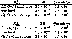
The results for  and
and  are displayed in
tables 4.5 and 4.6, respectively. For comparison, the
tree level branching ratios of table 4.1 and the rates for
the amplitudes without the loop contributions are also shown. The
separation between loop and counterterm contributions is of course
scale dependent. This scale dependence is absorbed in the scale invariant
constants
  defined in Eqs.(4.20),
(4.23). In other words, the entries in tables 4.5,
4.6 for the amplitudes without loops correspond to setting
all coefficients
  in tables 4.3,
4.4 equal to zero.

Table 4.5: Branching ratios and expected number of events at DA NE
for
  .
.

Table 4.6: Branching ratios and expected number of events at DA NE
for
  .
.