 ,
,  final states,
leads to the determination of both
 and
and  .
.
As extensively discussed, for example in Refs. [3,19,20],
the study of the time difference distribution, for
 ,
,  final states,
leads to the determination of both
 and
and  .
.
Introducing as usual the amplitudes

eq. (8), integrated over the pion phase space, gives:
If  there is an asymmetry between the events
with positive and negative values of t:
neglecting in eq. (11) terms proportional to
 ,
the
,
the  and
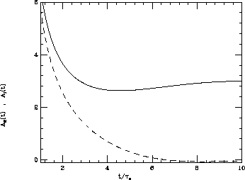
and  coefficients, shown in Fig.1, are given by:
It can be seen that  becomes nearly
independent of t, and equal to 3, for
  ; on
the other hand
  is strongly dependent on t and
vanishes for
  .
.

Figure 1: Coefficients of  (full line)
and
  (dashed line) defined in eq.(11).
Therefore a measurement of the asymptotic value
of  or of the value of the integrated asymmetry

allows a clean determination of
 . The statistical error on A
is
given by:

where N is the number of  events.
At the reference DA
 NE luminosity the statistical error on
 is then:

The integrated asymmetry A allows a precise determination of
 but gives no information on the imaginary part of
 .
To overcome this problem a further method can be exploited to measure both
 and
and  from the
 decay time difference:
the experimental distribution
![]() can be fitted by the theoretical distribution of
eq. (10), and
can be fitted by the theoretical distribution of
eq. (10), and  and
and
 can be used as free parameters of the fit.
It must be stressed that this procedure is very sensitive to the
experimental resolution on the measurement of d.
The information
contained in the shape of the
 distribution can be easily washed out, in particular
in the region of interest for the determination of
  ,
where
  . In fact only in this range of d
values
  is different from zero and the strongly varying
behaviour of
  can be smeared out by a bad vertex
reconstruction.
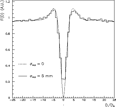
This effect is shown in Fig. 2, where the theoretical distribution is compared
with a simulated experimental distribution with a Gaussian error on the d
measurement equal to 5 mm.
can be smeared out by a bad vertex
reconstruction.
This effect is shown in Fig. 2, where the theoretical distribution is compared
with a simulated experimental distribution with a Gaussian error on the d
measurement equal to 5 mm.![]()

Figure 2: Comparison between the theoretical F(d) distribution
for  and that
obtained with an experimental vertex resolution
  .
.
The effects of the finite experimental resolution have been
discussed, for example in [20], to which we refer.
The results of the quoted analysis are that the determination of
 is practically unaffected by the experimental resolution,
while the statistical error on
  increases by more
than a factor 2.
This analysis estimates that the accuracy achievable
for a realistic detector is:

These numbers have to be compared with the present experimental situation shown in the introduction.